The agent wants one big table

9 Jul 2026

The Scout Agent on my FPL project (Fantasy Premier League, the official fantasy football game: pick a squad of real players, score points from their real performances) plans its own data access. You ask it whether to captain Haaland or Palmer this week, the planner turns that into a handful of tool calls, the tools fetch, and the agent reasons over whatever comes back before it commits to an answer. Building it, I made one decision early that I didn’t think hard about and now think was the most load-bearing one on the whole data side: every tool returns a flat, pre-joined record. One player, one object, with form and fixtures and injury signal and sentiment already stitched together. The agent never joins anything itself.

That wasn’t foresight. It fell out of the pipeline shape, because the enrichment step already produces one curated record per player, so the agent-facing tools just hand that back. But watching the agent work, I’ve become convinced the flatness is doing more than saving a query. It’s making the agent correct more often.

I meet the same question from the other side in the platform work I do professionally, building analytics serving layers that now have to answer both a dashboard’s queries and, increasingly, an agent’s. Same problem, higher stakes: how do you shape data for a query engine and a language model at once. FPL is just the version small enough that I could watch the whole thing with my own hands on the keyboard. And I think it’s a small instance of something the whole analytics world is bumping into in 2026: LLM agents are a forcing function for denormalisation, for a reason the old denormalisation arguments never had.

Denormalisation isn’t new, and the pendulum was already mid-swing before agents showed up. The relational orthodoxy (normalise until it hurts, join at read time) was built for a world where storage was expensive and writes had to stay consistent. Kimball’s dimensional modelling was the first big concession on the analytics side: facts in the middle, dimensions around them, a star you join at query time, denormalised enough to be fast but structured enough to govern. Columnar warehouses pushed it further. Once storage is cheap and the engine is columnar, the case for the join weakens, and the One Big Table pattern (flatten the star into a single wide table, eat the storage, delete the joins) starts winning on raw scan performance. The numbers people quote for the switch are real if unspectacular; Fivetran put it at 25 to 50 percent depending on the warehouse. Worth doing, not worth a blog post.

The agent reason is different in kind, and it’s the one I find genuinely interesting. When an LLM writes SQL, or plans a sequence of data fetches, the joins are where it goes wrong. Not the aggregations, not the filters, the joins. It has to hold the foreign-key graph in its head, pick the right join path, avoid the fan-out that silently double-counts, and it does all of that from a schema description in its context window rather than from having lived in the data. A human analyst learns the traps once and remembers them. The model rediscovers them, or doesn’t, on every query.¹

Give it one wide table and most of that failure surface disappears. There’s no join path to choose because there’s no join. The schema it has to reason about is one relation, however wide it gets. Text-to-SQL accuracy against a single denormalised table is markedly better than against a normalised schema for exactly this reason, and it’s why so much of the natural-language-query and agent tooling springing up this year keeps landing on a flat serving layer underneath. That buys scan speed, as it always did, but it now also buys something the old argument never mentioned: whether the model gets the question right at all. We denormalised for the engine for a decade. Now we’re denormalising for the reader, and the reader is a language model.

Start with the raw speed, because it’s the part that’s easy to measure and hard to argue with. Postgres stores each row’s fields together on disk, which is exactly right when you’re fetching or updating whole records and exactly wrong when you’re scanning one column across millions of rows to aggregate it. The analytical query touches a few columns; the row-store still walks past every other field of every row to reach them. A columnar engine stores each column contiguously, reads only the columns the query names, and runs the scan through a vectorised executor that chews through chunks with SIMD. On the public ClickBench suite, analytical queries that take Postgres tens of seconds to minutes come back from a columnar engine in milliseconds to low single digits, commonly 10 to 100 times faster, depending on whether Postgres can lean on an index or is forced into a sequential scan. Put a wide, denormalised table under that engine and the join cost comes off on top of the scan cost.

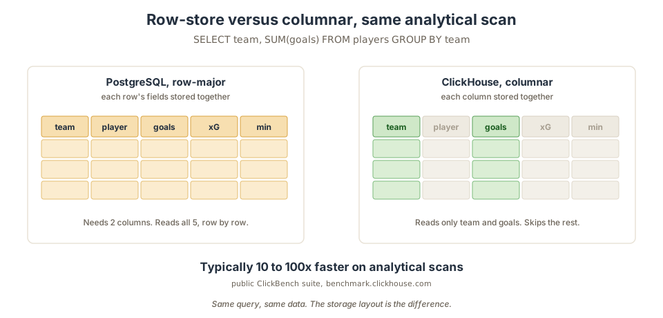
ClickHouse is the engine I reach for here, because its design leans into this shape rather than tolerating it. Its own guidance on denormalisation is unusually candid for vendor docs: denormalise the things that don’t change often, keep the join for the things that do. The wide MergeTree table is the default idiom, not an exception you engineer around. Materialised views give you a place to put the flattening so it happens on write, incrementally, rather than in the serving path where the agent is waiting. And the native array, tuple and map types let you fold a short list of tags or categories onto the row without either a join or a second table, which is the thing a normalising purist finds most offensive and an agent finds easiest to query.

The clearest public example of the pattern living under an AI product is Langfuse, the LLM-observability tool. They run their agentic-era analytics on ClickHouse Cloud precisely because agent traces are high-volume, wide, and queried under concurrency by dashboards and, increasingly, by other agents. I use Langfuse on the FPL pipeline for tracing, so I met their architecture from the consumer side first. It was only later I clocked that the reason it stays fast under that load is the same reason my agent’s flat player records stay easy to reason about.

None of this means the star schema is finished, and I’d push back on anyone who says it is. Denormalisation moves cost, it doesn’t remove it. The moment you flatten, a correction to one dimension value becomes a rewrite across every row that carried it, and the wide table stops being a convenient truth and starts being a maintenance liability if you treat it as the system of record. The shape that actually holds up is the one the more careful practitioners have been describing all year: a normalised, governed model as the system of record, feeding a denormalised serving layer built for how the data is consumed. dataarchitect.studio frames it cleanly, the OBT is derived from the dimensional model, not a replacement for it. You keep the star where truth and corrections live, and you materialise the flat table the agent reads. Two layers, different jobs.

Which is, more or less, what I stumbled into on FPL without the vocabulary for it. The structured player and fixture data lives upstream; the agent reads a flattened, pre-joined record that gets rebuilt when the upstream changes. I didn’t design it that way because I’d read the theory. I designed it that way because the agent was better when I did, and the theory turned out to be waiting for me when I went looking for why. The professional version of the same split is more deliberate and higher-stakes; FPL is where I first saw it work.

The part I didn’t expect is how cleanly the two reasons stack. The engine wanted flat data for speed and got it a decade ago. The model wants flat data for comprehension and is getting it now, off the same table. When one design decision pays off twice for unrelated reasons, it’s usually structural rather than lucky.